Overview
Switching from the raster package to terra for spatial analysis
Thu, Aug 25, 2022
Spatial data in R has a reputation for being tedious and time consuming. With so many different spatial file types (.shp, .nc, .gpkg, .geojson, and .tif to name a few) with various resolutions and coordinate reference systems, it can be challenging to produce accurate maps. Most data scientists have historically utilized the raster package to calculate cell values across stacked layers and recognize patterns over space and time. In pursuit of improving methodology and keeping up with the hip trends in environmental science, many scientists are motivated to make the spatial switch from raster to terra. The terra package is essentially the modern version of raster, but with faster processing speeds and more flexible functions.
Some examples of similar functions between raster and terra are as follows:
| raster | terra | Use |
|---|---|---|
| raster() | rast() | Rasterize a spatial file (such as a .tif or a spatial dataframe) into a rasterLayer (for the raster package) or spatRaster (for the terra package) |
| stack() | rast(), c() | Create raster stack to execute calculations across layers. terra::rast() is a more broadly applicable function since it can detect the quantity of spatRasters present as .tif files in a directory, then automatically stacks them. Alternatively, if the files have already been read in as spatRasters, use c() to stack them and assign the stack to a new object name. |
| calc() | app(), lapp(), focal(), etc. | Execute a function across a raster or raster stack. terra has multiple functions with varying degrees of flexibility depending on if the function is applied across layers, and if the same function is applied to each layer. |
| resample() | resample() | Convert the origin and/or resolution of a raster to that of another. For example, you might want to add two rasters, but need to convert the first raster from a resolution of 0.5 degrees to 0.01 degrees to match the higher resolution of the second raster. |
| extract() | extract() | Pull values from a raster object where they intersect the locations of another spatial object, such as points that fall within polygons. For raster(), the spatial objects can be points, lines, and polygons. For terra, the second spatial object must be a vector or matrix/dataframe of coordinates. For example, the spatial object from which we are extracting is a geometry columns of polygons, the user cannot input the entire spatial dataframe, but rather needs to vectorize the geometry column of the polygons using terra::vect() then input that object into terra::extract(). |
| aggregate() | aggregate() | Combine cells of a raster to create a new raster with a lower resolution. Aggregation groups rectangular areas to create larger cells. The value for the resulting cells is computed with a user-specified function. This is also know as down-sampling. |
| freq() | freq() | Create a frequency table of the values of a raster. |
Let’s take a look at how we converted our workflow to calculate global soft bottom habitat destruction through the years 2012-2020.
Soft Bottom Habitat Destruction
The Ocean Health Index (OHI) uses various spatial datasets to monitor the relationship between the health of marine systems and human well-being for 220 regions around the world. The way OHI historically calculated soft bottom habitat destruction was by using annual fisheries catch data as a proxy for trawling and dredging activity, because these types of fishing severely disturb benthic habitat. The fisheries catch data was rasterized and overlaid onto polygons of exclusive economic zones for all OHI regions, then spatially standardized by summing each fishing coordinate within the exclusive economic zone and dividing that sum by the square kilometers of softbottom habitat.
In 2022, OHI switched the data source from fisheries catch to apparent fishing effort for trawling and dredging from Global Fishing Watch using their new user-friendly API. This data comes in units of hours of apparent fishing effort associated with the coordinate, geartype, and year of each observation. We used the Global Fishing Watch API to pull codes for all the exclusive economic zones for the 220 OHI regions, then pulled apparent fishing effort for each exclusive economic zone from 2012-2020.


Expand to see the Global Fishing Watch API in action
# iterate through all EEZ codes for all regions to extract apparent fishing hours:
for(i in regions) {

  # create dataframe that contains the column `id` that is list of all EEZ codes for one region
  eez_code_df <- get_region_id(region_name = i, region_source = 'eez', key = key)

  # convert that column into a numeric list of EEZ codes to feed into the next loop:
  eez_codes <- eez_code_df$id

  print(paste0("Processing apparent fishing hours for ", i, " EEZ code ", eez_codes))

  for(j in eez_codes) {
    fishing_hours <- gfwr::get_raster(spatial_resolution = 'high', # 0.01 degree resolution
                                      temporal_resolution = 'yearly',
                                      group_by = 'flagAndGearType',
                                      date_range = '2012-01-01,2020-12-31',
                                      region = j,
                                      region_source = 'eez',
                                      key = key) %>%
      # rename columns for clarity:
      rename(year = "Time Range",
             apparent_fishing_hours = "Apparent Fishing hours",
             y = Lat,
             x = Lon,
             geartype = Geartype) %>%
      # keep track of the administrative country for each EEZ
      mutate(eez_admin_rgn = i) %>%
      select(year, apparent_fishing_hours, y, x, eez_admin_rgn, geartype)

    print(paste0("Extracted all apparent fishing hours for ", i, " EEZ code ", j))

    write_csv(fishing_hours, paste0(filepath, i, "_", j, "_effort.csv"))
  }
}
While initially cleaning the Global Fishing Watch data, we separate it into different dataframes for trawling and dredging since we need to process the geartypes differently. In order to convert the fishing effort coordinates into annual spatRasters, we use the following approach:
years = as.factor(2012:2020)

for(i in years){
  # trawling data:
  trawl_annual_raster <- fish_effort_trawl_annual %>%
    dplyr::filter(year == i) %>%
    dplyr::select(-year) %>%
    terra::rast(type = "xyz", crs = "EPSG:4326", digits = 6, extent = NULL)

  filename <- paste0("fish_effort_trawl_", i, ".tif")

  # save annual raster file for trawling:
  terra::writeRaster(
    trawl_annual_raster,
    filename = paste0(filepath, i, filename),
    overwrite = TRUE
  )
}
terra processes this dataframe into a spatRaster object because we simplified it into just 3 columns: x, y, and fishing effort, and with the argument type = "xyz" we specified that there’s an x value, y value, and other value (z) at that coordinate. Note that the WGS84 coordinate reference system is specified using the simple "EPSG:4326" syntax, rather than the complex proj4 format that raster::raster() prefers: "+proj=longlat +datum=WGS84 +ellps=WGS84 +towgs84=0,0,0". We run the same code for the dredging dataframe.
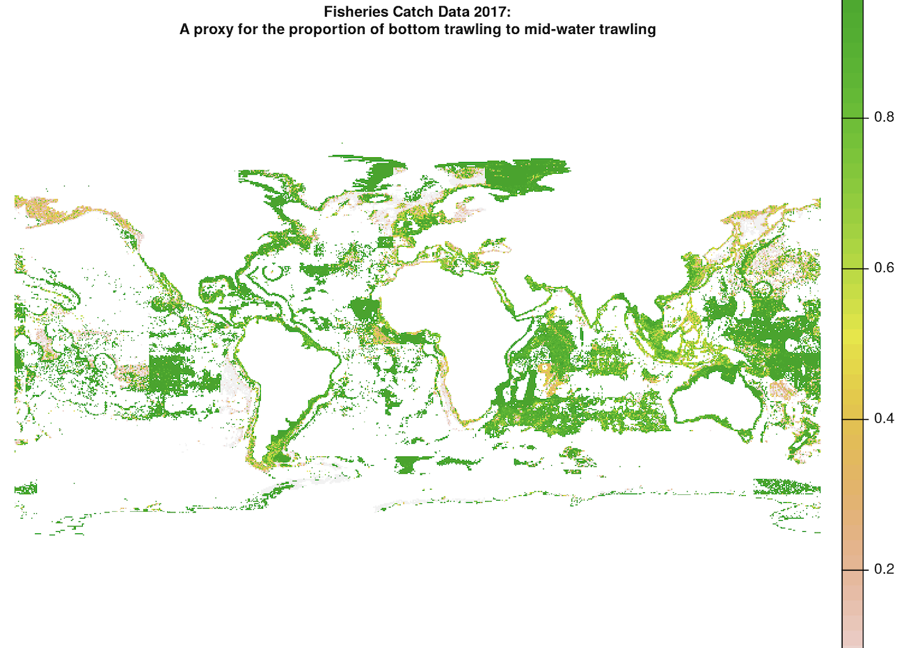
Next, we subset the trawling data by filtering for just bottom trawling and exclude mid-water trawling, since bottom trawling is the method that damages the seafloor. In order to do this, we multiply the trawling effort spatRaster by another spatRaster that represents the proportion of bottom trawling to mid-water trawling at each coordinate, provided by Watson and Tidd (2018). The raw trawling proportion raster has many NA values:
In order to multiply these spatRasters, we first want to interpolate the bottom trawling proportion raster as accurately as possible. This interpolation takes 2 steps:
1. Use the local mean of surrounding cells to fill in NA values (nearest neighbor) using terra::focal().
trawl_depth_proportion_interpolated <- terra::focal(
  x = trawl_depth_proportion,
  w = 5, # sets a 5 cell window around NA pixel
  fun = "mean",
  na.policy = "only", # only interpolate NA values
  na.rm = T,
  overwrite = TRUE
)
2. Interpolate all remaining NA values using the terra::global() function.
global() can be used similarly to terra::app() for simple functions, such as calculating the mean of all non-NA values in the entire raster layer:
global_trawl_proportion_avg <- terra::global(
  trawl_depth_proportion_interpolated,
  fun = "mean",
  na.rm = TRUE
)

trawl_depth_proportion_interpolated[is.na(trawl_depth_proportion_interpolated)] <- global_trawl_proportion_avg[1,1]
In order to check if any NA values remain, we can use the isNA function in terra::global() that returns the sum of all NA values in the spatRaster:
terra::global(
  trawl_depth_proportion_interpolated,
  fun = "isNA"
)
An output of 0 informs us we have successfully interpolated all NA’s!
The fully interpolated and resampled map for trawling proportion looks like this:
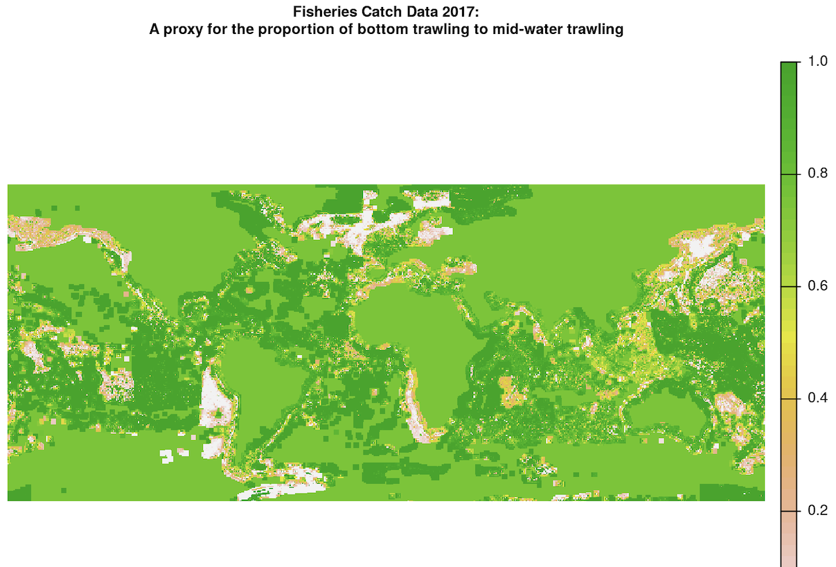
The continental raster cells were originally NA values, and we used terra::global() to fill them in with the mean value in our last interpolation step. While it does not make logical sense to assign land value with a trawling proportion value greater than 0, this is useful for our use case because the only purpose of this trawling proportion raster is to retain the trawling fishing effort values in the other raster and subset many of them to a smaller value if the proportion is less than 1 in this interpolated raster. As a result, all the land cells that have a value of 1 in the interpolated raster will be multiplied by NA in the fishing effort raster, so they will not be counted in the final fishing effort scores.
Next, we check the raster’s resolution, extent, and other characteristics by calling the raster object and viewing the output:
class       : SpatRaster
dimensions  : 360, 720, 1  (nrow, ncol, nlyr)
resolution  : 0.5, 0.5  (x, y)
extent      : -180, 180, -90, 90  (xmin, xmax, ymin, ymax)
coord. ref. : lon/lat WGS 84 (EPSG:4326)
source      : bottom_trawl_prop_2017.tif
name        : bottom_trawl_prop_2017
min value   :                      0
max value   :                      1
Note that the resolution is 0.5 degrees. We want to up-sample this spatRaster to increase the resolution to that of the fishing raster, which is 0.01 degrees. We can do this by using the trawling effort raster as a template resolution in the resample() function:
# resample the interpolated trawling proportion data
# match the resolution of the GFW fishing effort data
trawl_depth_proportion_resampled <- terra::resample(
  x = trawl_depth_proportion_interpolated,
  y = fish_effort_trawl, # use the GFW data as the sample geometry
  method = "near" # nearest neighbor calculation to up-sample
)
We can check that the resolution was increased to 0.01 degrees by calling the name of the raster again to view the adjusted raster characteristics:
class       : SpatRaster
dimensions  : 14930, 36001, 1  (nrow, ncol, nlyr)
resolution  : 0.01, 0.01  (x, y)
extent      : -180.005, 180.005, -67.315, 81.985  (xmin, xmax, ymin, ymax)
coord. ref. : lon/lat WGS 84 (EPSG:4326)
source      : trawl_depth_proportion_resampled_2017.tif
name        : focal_mean
min value   :          0
max value   :          1
Great!
Next, we need to match the spatRaster extents, which is the minimum and maximum coordinates in both the x and y directions (xmin, xmax, ymin, ymax). We use terra::extend() for this. First extend one spatRaster to the extent of the other, and then vice versa to ensure that each of the four dimensions are maximized and consistent with the other spatRaster. If we were to use the raster package, the equivalent (but slower) function goes by the same name. Both packages also have the function crop() that reduces the extent of a larger raster to that of a smaller raster.
trawl_depth_proportion_extended <- terra::extend(
  trawl_depth_proportion_raster,
  fish_effort_raster
)

fish_effort_extended <- terra::extend(
  fish_effort_raster,
  trawl_depth_proportion_extended
)
In order to check if the extents match, we can use terra::compareGeom() to return TRUE or FALSE:
terra::compareGeom(
  fish_effort_extended,
  trawl_depth_proportion_extended,
  stopOnError = FALSE # makes the function return FALSE if the extents are different
)
There is no direct equivalent raster function for terra::compareGeom(), and it’s quite handy!
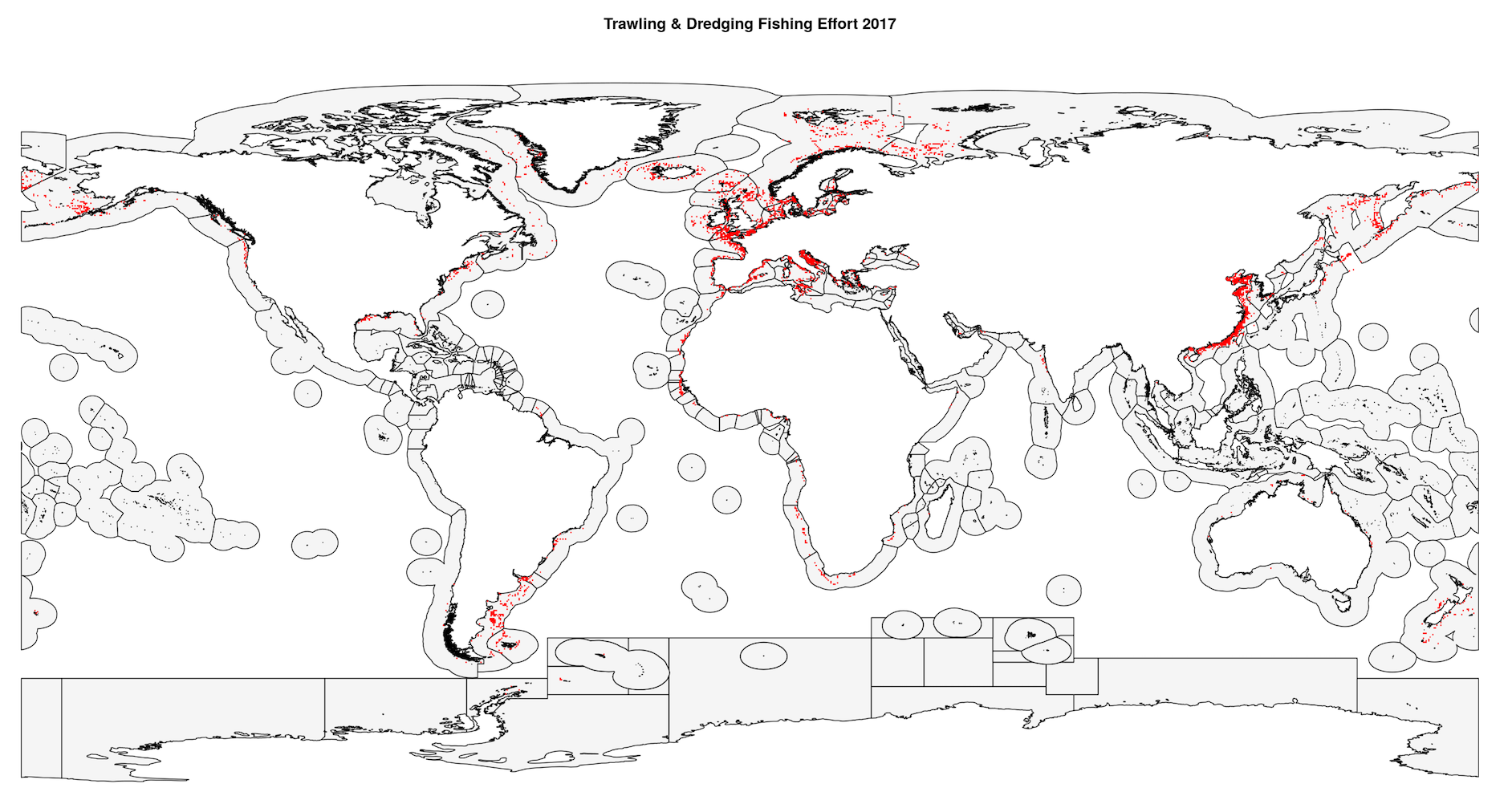
The 2017 map of fishing effort looks like this:
Next, we use writeRaster() to re-write the two extended spatRasters as .tif files to the same directory so we can read them in as spatRasters in our next loop.
The last step before multiplying the spatRasters is to stack them. With the raster package, we would use stack(). With terra, we simply read in the spatRasters simultaneously from the same directory using the familiar function rast() and the result is a spatRaster object with two layers that have matching resolutions, origins, and extents!
# define the 2 raster filepaths as an object
rasters <- here::here('data', 'int', 'fish_effort_annual', 'trawling', i, 'extended') %>%
  list.files(pattern = ".tif", full = TRUE)

# stack the spatRasters, with each spatRaster representing 1 layer:
trawl_stack <- terra::rast(rasters)
Finally, it’s time to multiply the spatRasters! There are a few options for multiplying, summing, taking the mean of two rasters, or executing custom functions in the terra package. For example, you could use app(), lapp(), sapp(), etc. You should choose your calculation function depending on:
- If you are calculating through layers, across only one layer, if you are using the same calculation on all layers or not (for example, if you have three layers you might execute
x * y * zorx * y + z) - If your function is simple (like “sum” or “mean”) or a complex custom function that would take much more compute to execute over a large, global
spatRaster.
Since we are working with only two layers and are executing a basic multiplication, we can use the simplest option: app() or have a little more fun with the syntax and use lapp() like so:
trawling_corrected <- terra::lapp(
  trawl_stack,
  fun = function(x,y){return(x*y)}
)
If we were working with rasterLayers in the raster package, we would have used the general function calc() for simple calculations.
After cleaning up the dredging spatRaster, we want to add the fishing effort associated with each cell to our corrected trawling raster, so we stack them as we did before and execute simple addition across layers:
all_fishing <- terra::app(
  effort_stack,
  fun = "sum",
  na.rm = TRUE
)
In order to pair the trawling and dredging fishing effort with the 220 OHI regions, we extract the trawling and dredging points from the exclusive economic zone polygons that are associated with each region. In raster and terra, we would use their respective functions both called extract(). terra::extract() allows for more flexibility in extracting the proportion of cells that fall within the polygons, if they are on the borders. However, our experience with these functions is that they are very slow to execute.
exact_extractr::exact_extract()offers much faster processing speeds, but requires different syntax. This function allows the user different options for the output that range in complexity. For example, one can extract a list of dataframes, each of which contains the cell values and weight (coverage proportion) for one polygon. The user can then use those values and weights as they want. Alternatively,exact_extract()can do a weighted calculation for us, with arguments that specfies a weighted function and the data to use as weights.
years_all <-  as.factor(2012:2020)

for (i in years_all) {

  print(paste("Processing ", i, " fishing effort."))

  # read in the annual fishing raster for all regions
  # this represents corrected trawling plus dredging data
  fishing_raster <- terra::rast(paste0(filepath, filename, i, ".tif"))

  # extract the fishing effort that falls within the polygons of OHI regions
  extracted <- exactextractr::exact_extract(fishing_raster, ohi_regions_filtered)

  # sum effort by polygon and append polygon dataframes into 1
  all_polygon_effort <- data.frame()

  for (j in seq_along(extracted)) {

    df <- extracted[[j]]

    weighted_effort_polygon <- df %>%
      # weight the fishing effort within each cell by the porportional coverage of the cell
      mutate(effort = value*coverage_fraction,
             polygon_id = j) %>%
      select(polygon_id, effort) %>%
      group_by(polygon_id) %>%
      summarize(effort_sum = sum(effort, na.rm = TRUE))
    # bind the polygon-specific sum to the master dataframe of polygon sums
    all_polygon_effort <- rbind(all_polygon_effort, weighted_effort_polygon)

  }

  # bind regional id's to the polygon id's
  rgn_id <- ohi_regions_filtered$rgn_id
  regional_polygon_effort <- cbind(all_polygon_effort, rgn_id)

  regional_polygon_effort <- regional_polygon_effort %>%
    group_by(rgn_id) %>%
    # combine each land and eez polygon for the same region
    # some of the fishing points landed just on the border of these polygons
    # meaning they are associated with land when they should be in the EEZ
    summarize(effort_sum = sum(effort_sum, na.rm = TRUE)) %>%
    mutate(year = i)

  # convert this raster info into a csv that represents fishing effort
  # for each OHI region for year i
  write.csv(regional_polygon_effort, file = paste0(filepath, filename, i, ".csv"),
  row.names = FALSE)
  print(paste0("Saved ", i, " fishing effort csv to ", filepath, filename, i, ".csv"))
}
That about covers it for fishing effort rasters. You can find the complete script here on the OHI github repository for the 2022 assessment. Please feel free to contact the OHI team with any questions or suggestions. For more spatial wrangling with terra, check out the upcoming blog post about our new tidal flats data layer!
References
-
Daniel Baston (2022). exactextractr: Fast Extraction from Raster Datasets using Polygons. R package version 0.8.2, https://CRAN.R-project.org/package=exactextractr.
-
Global Fishing Watch. [2022]. www.globalfishingwatch.org
-
Hijmans R (2022). terra: Spatial Data Analysis. R package version 1.6-3, https://CRAN.R-project.org/package=terra.
-
R Core Team (2022). R: A language and environment for statistical computing. R Foundation for Statistical Computing, Vienna, Austria. URL https://www.R-project.org/.
-
Watson, R. A. and Tidd, A. 2018. Mapping nearly a century and a half of global marine fishing: 1869–2015. Marine Policy, 93, pp. 171-177. (Paper URL)
-
Wickham H, Averick M, Bryan J, Chang W, McGowan LD, François R, Grolemund G, Hayes A, Henry L, Hester J, Kuhn M, Pedersen TL, Miller E, Bache SM, Müller K, Ooms J, Robinson D, Seidel DP, Spinu V, Takahashi K, Vaughan D, Wilke C, Woo K, Yutani H (2019). “Welcome to the tidyverse.” Journal of Open Source Software, 4(43), 1686. doi:10.21105/joss.01686 https://doi.org/10.21105/joss.01686.
This post was created by the 2022 OHI Fellows.