The Trouble with Transformation

The Challenges of Projecting Spatial Data

by Anna Ramji

Fri, Sep 13, 2024

Introduction

Have you ever wondered what happens to your mapped raster data when you project it from one Coordinate Reference System (CRS) to another? Or whether anything can go wrong when projecting?

In this article, we’ll walk through how reprojecting and transforming geospatial data can potentially lead to large errors! To help you avoid this problem we’ll show you how to check for and avoid these problems.

To demonstrate these ideas, we’ll look through a fairly straightforward example using commercial landings data (Watson, 2017).

Coordinate Reference Systems

It’s important to understand at least a little bit about coordinate references systems before we move on. A previous OHI News post by Dustin Duncan delves into details about coordinate reference systems, projections, and more. For now, we can think about coordinate reference systems as a way to describe locations in a standardized way such that a 2-dimensional point on a projected map describes a “real” position on Earth.

Packages Used

library(here) # for reproducible file paths
library(terra)  # for geospatial data
library(tidyverse) 

Data Exploration

Overview

To begin, we will read in the data and familiarize ourselves with some of the basic information relevant to geographic data, particularly the coordinate reference system and the areas represented by each raster cell. We will then create exploratory data visualizations and perform some investigations of raster cell size and raster values.

Process

We’ll read the raster into R using {terra}’s rast() function and the {here} package.

# Read in commercial landings data
fish <- terra::rast(here::here("Reference", "CRS", "commercial_landings_2017.tif"))

When working with new data, it is important to start with a preliminary exploration of the data. Here we’ll print out basic information about our spatial object, fish.

# print out geospatial data info (class, dimensions, resolution, extent, CRS, etc.)
fish

class       : SpatRaster 
dimensions  : 347, 720, 1  (nrow, ncol, nlyr)
resolution  : 0.5, 0.5  (x, y)
extent      : -180, 180, -85.5, 88  (xmin, xmax, ymin, ymax)
coord. ref. : lon/lat WGS 84 (EPSG:4326) 
source      : commercial_landings_2017.tif 
name        : commercial_landings_2017 
min value   :                      0.0 
max value   :                 145169.4

This spatial object’s coordinate reference system (CRS) – printed on the coord. ref. : line – is WGS 84 (EPSG:4326), which is a geographic CRS used by Google Earth and is the native system of Global Positioning Systems (GPS). WGS 84 refers to the datum World Geodetic System 1984 ensemble, which specifies that the WGS 84 ellipsoid is used. EPSG 4326 defines the full CRS using the WGS 84 ellipsoid, and it is the horizontal component of the 3-dimensional system. The lon/lat text before WGS 84 in the output indicates that we are dealing with a geographic coordinate system with angular units (degrees) of latitude and longitude.

This is our initial geographic CRS, and any changes we make to this down the line will involve projecting and transforming the data.

The dimensions field indicates that there are 347 rows (nrow), 720 columns (ncol), and only 1 layer (nlyr), which we know is tonnes of commercial fisheries landings in 2017.

The name field indicates that the raster has one layer, named “commercial_landings_2017”. The min value and max value fields indicate that across all raster cells in this layer, the minimum value is 0 and the maximum value is 145169.4.

Another important aspect of a raster’s structure is its resolution. Resolution describes the amount of Earth’s area that each grid cell represents. When a raster has more cells, the data will have a finer, more detailed resolution. One interesting thing about lon/lat coordinate reference systems is that the cells represent different amounts of area. This has all sorts of implications for how we interpret visualizations of the data!

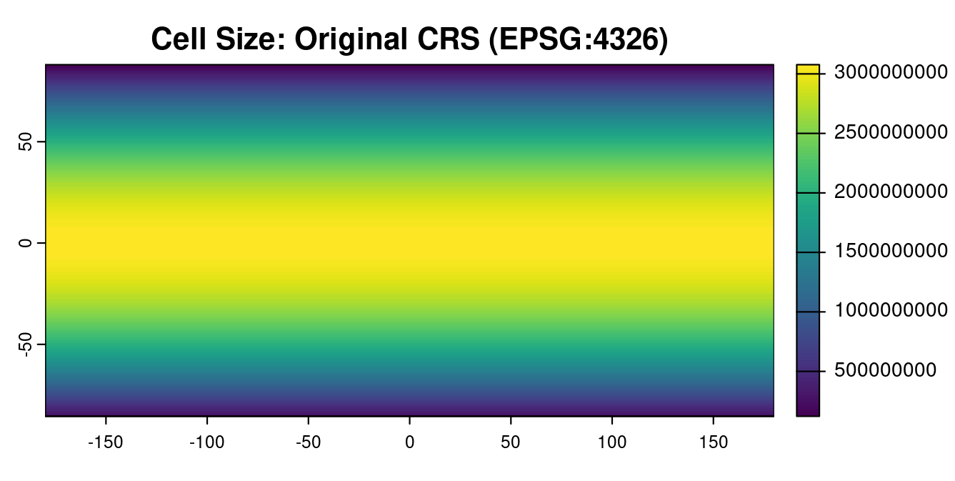
To understand more about how cell area varies in the original CRS’s extent, we will use terra::cellSize() and plot the cell area with respect to latitude.

cell_area <- terra::cellSize(fish)
terra::plot(cell_area,
	     # set title
     main = "Cell Size: Original CRS (EPSG:4326)")

print(cell_area)

class       : SpatRaster 
dimensions  : 347, 720, 1  (nrow, ncol, nlyr)
resolution  : 0.5, 0.5  (x, y)
extent      : -180, 180, -85.5, 88  (xmin, xmax, ymin, ymax)
coord. ref. : lon/lat WGS 84 (EPSG:4326) 
source(s)   : memory
varname     : commercial_landings_2017 
name        :       area 
min value   :  122442386 
max value   : 3077249667 
	

The summary output shows that area represented by each raster cell ranges from 122 million square meters (m²) to 3 billion m². We confirmed that these were in square meters with terra::crs(). We also summed the total global area using terra::expanse() on the cell_area object, and obtained a total calculated surface area of around 509 trillion, which is similar to Earth’s 510 trillion m² area.

The plot shows us that the raster cells do not represent the same area across the globe. As we move from the equator to the poles, the area that raster cells represent decreases significantly.

This is notable for several reasons:

• The poles will be over-represented in any visual representation of these data. This is why Greenland looks so large in many maps – it is often visually represented to have the same area as Africa, when in reality Africa is over 14 times larger.

• The data will be misleading if the values are counts, e.g., tonnes of fish, number of people, etc.. For example, imagine that fish population densities are constant throughout the oceans (which is obviously not true). If this density data is converted to counts data, the extremes of the Northern and Southern Hemispheres will have lower counts because they represent less ocean area.

• This inconsistency in cell area may also hide some higher values near the equator, as each of those larger raster cells appear as uniformly sized pixels when plotted with the rest of the data.

Now that we understand more about the map architecture, we can explore the data within it!

We can use summary(fish) for a basic statistical summary of the map’s values:

# print out summary of value layer
summary(fish)

 commercial_landings_2017
 Min.   :     0.00       
 1st Qu.:     2.43       
 Median :    22.25       
 Mean   :   651.53       
 3rd Qu.:    84.65       
 Max.   :125112.30       
 NA's   :47150 

And we can use terra::plot() to visualize the data:

# basic plot
terra::plot(fish)

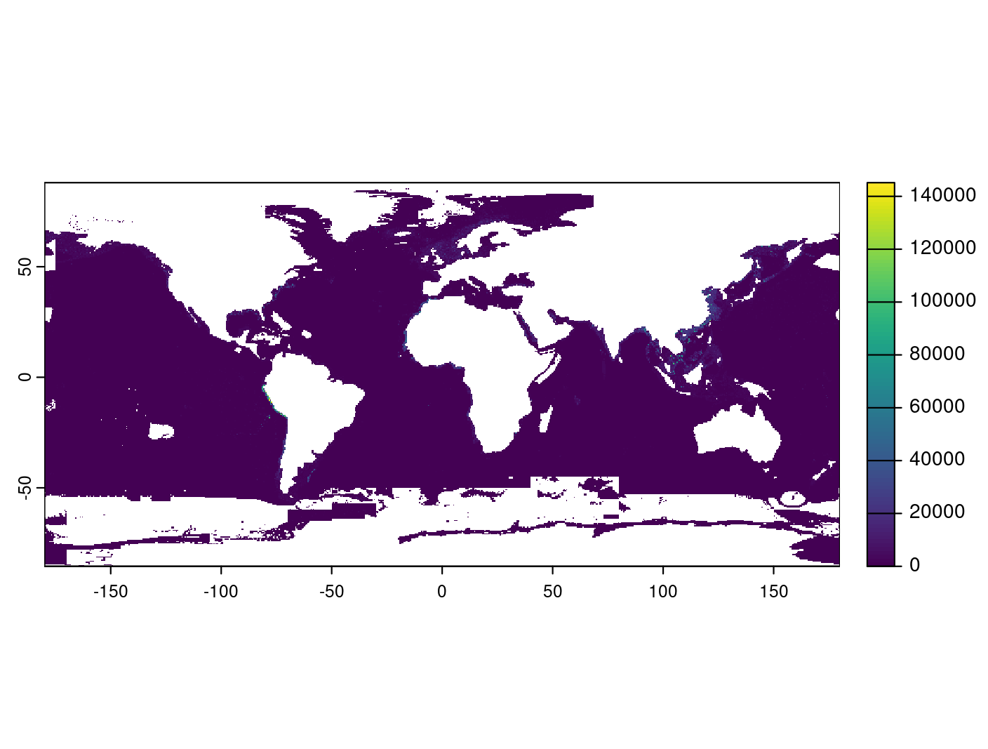
This plot is not very helpful for visualizing general patterns in landings because a few very large values of landings are making the smaller values difficult to see. We can log-transform the data to get a better look at what’s going on:

# log-transform and plot 
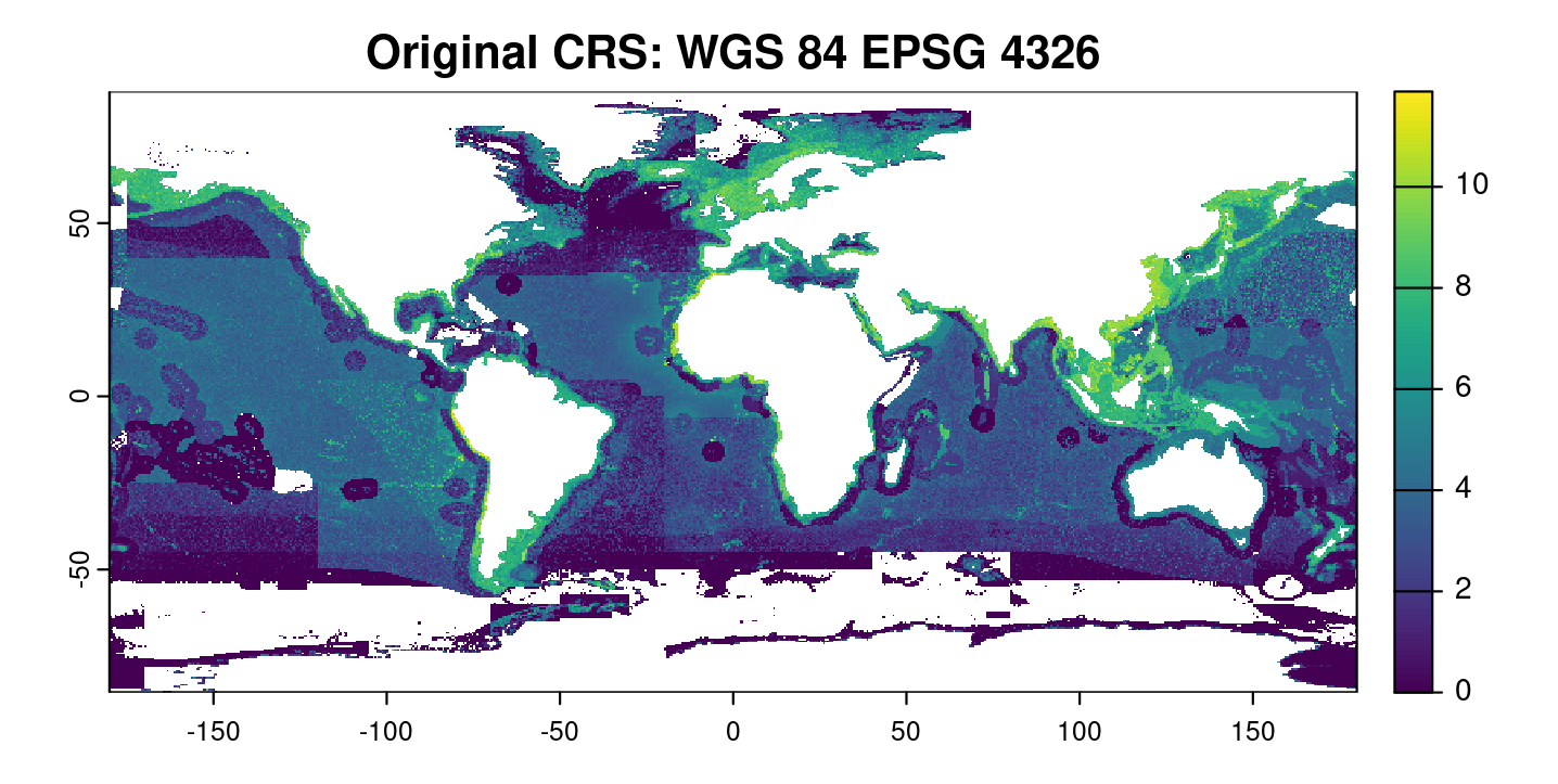
terra::plot(log(fish + 1),  main = "Log-transformed Commercial Landings (EPSG:4326)")

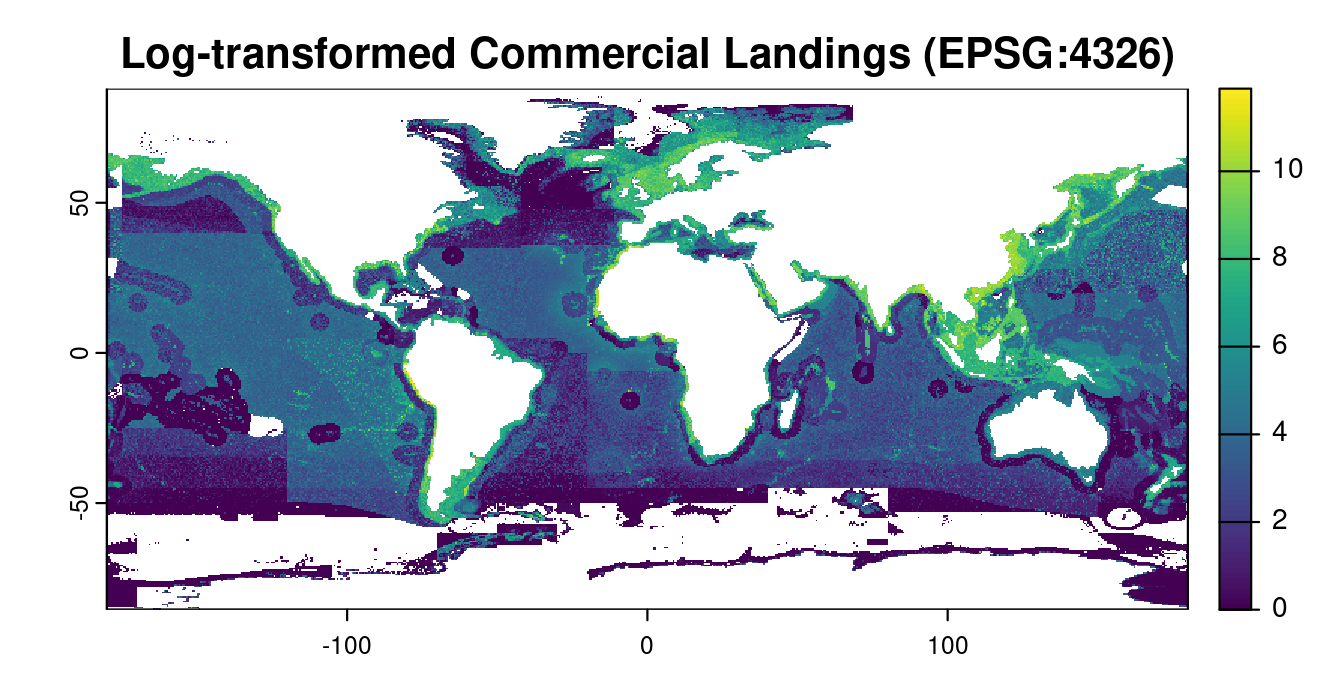
According to this visualization, there are more fisheries landings closer to coasts, with notable aggregations around Northern Europe, East and Southeast Asia, and Alaska.

These general patterns make sense given what we know about fisheries, but we also want to further confirm that we understand the map values and that the units make sense, i.e., tonnes, rather than kilotonnes.

One way to do this is to see how many tonnes of fish were caught globally in 2017 and compare this to a secondary dataset. To sum all values across all cells in the layer, we can use a global summary statistic (sum within terra::global()).

# global operation: sum
terra::global(fish, "sum", na.rm = TRUE)
#> 86.3 million tonnes

                               sum
<dbl>
commercial_landings_2017	86331119	

Does this value make sense?

To get a rough idea of whether the estimate of 86.3 million tonnes of commercial landings is sensible, we looked at Sea Around Us’s Tools & Data page, selecting Fishing sector for the dimension, as shown in the screenshot below.

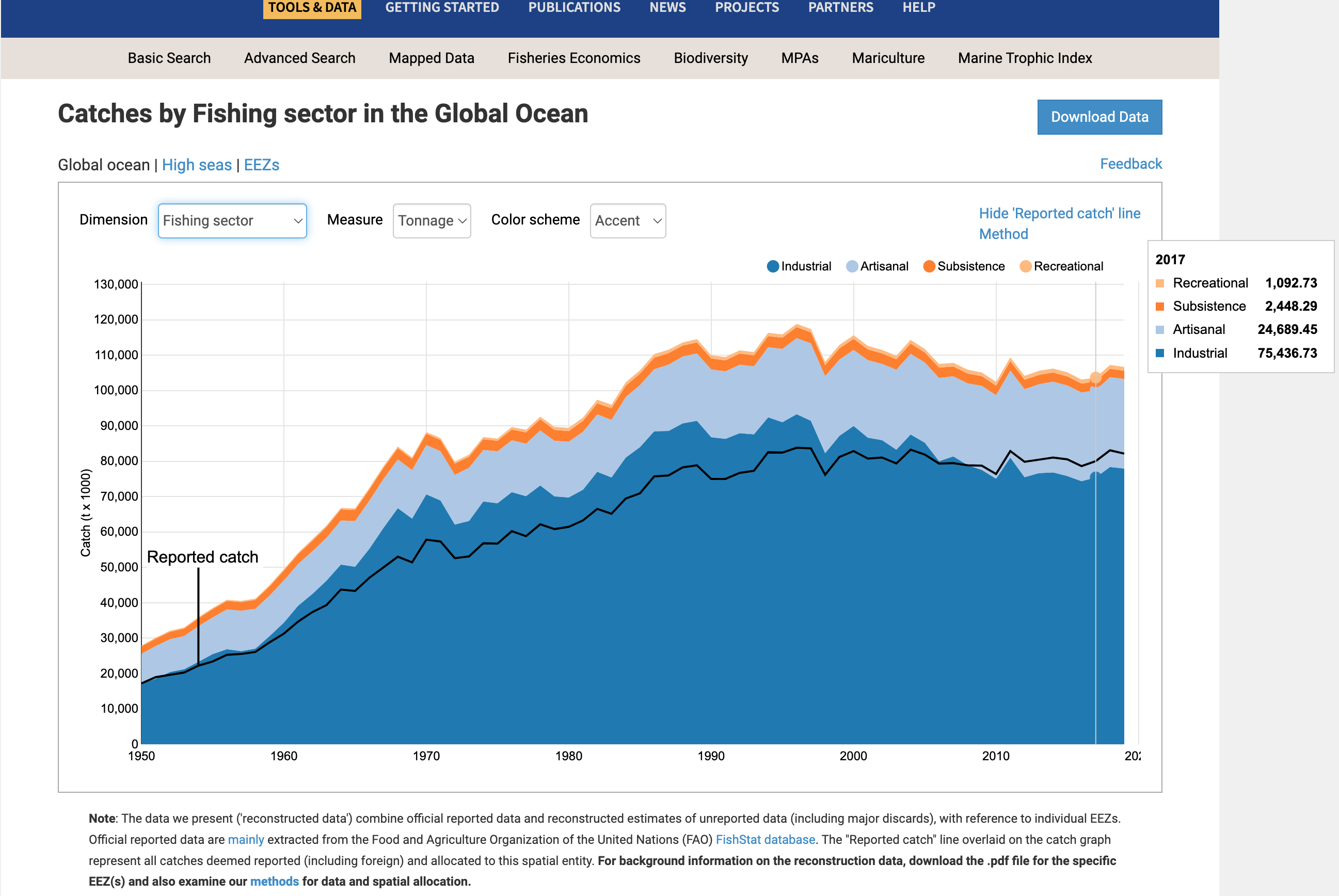
The Sea Around Us data reports about 80 million tonnes, which is somewhat less than what we report (86.3 million); however, this seems reasonable considering differences in methodology. For example, our data is configured a bit differently from the SAUP data in that we included Illegal, Unreported, and Unregulated landings (IUU) in landings. This and other differences can easily lead to this level of difference, and regardless, we can assume that this is close enough to seem like a reasonable value. An example of a value that wouldn’t make sense in this context is one in a different order of magnitude, such as 1 billion, 10 thousand, or potentially 100 million above or below this estimate.

CRS Projection: Mollweide

Overview

After getting a better understanding of these data, we want to see how projecting it to a new CRS will alter the data. Specifically, we will project the data from EPSG:4326 to Mollweide and investigate how this alters the data through exploratory analyses of the raster framework and data. SPOILER ALERT: Because we are working with count data (i.e., tonnes), this will result in an error!

We often use the Mollweide projection in our research because it is an equal area projection that is easier to work with and does not visually distort the significance of the poles.

Process

In the code chunk below, we’ll project the CRS from WGS 84 (EPSG:4326) to Mollweide – the projected CRS used in most OHI rasters. We’ll also plot the log-transformed projected data, as we saw when visualizing the data earlier, the non-transformed data is not very helpful for visualizing general patterns.

# define Mollweide CRS specifications
moll <- "+proj=moll +lon_0=0 +x_0=0 +y_0=0 +datum=WGS84 +units=m +no_defs"

# project data to Mollweide
fish_moll <- terra::project(fish, terra::crs(moll))

# Let's plot to see how this transformation impacted the data!

# plot data projected to Mollweide
terra::plot(log(fish_moll + 1), main = "Transformed CRS: Mollweide")

# compare to original CRS
terra::plot(log(fish + 1), main = "Original CRS: WGS 84 EPSG 4326")

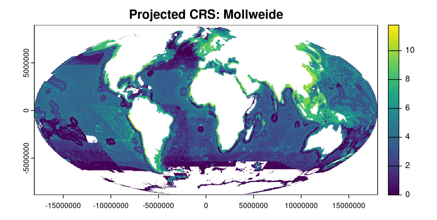
When looking at the Mollweide plot, even when comparing it to the plot of the data in its original CRS, the values don’t appear to have changed dramatically. We can see that the shape is quite different though – we’ve gone from a rectangle to an oval, and can see the warping and changes around the edges, especially at the polar extremes. There are still aggregations of higher values around the coasts of Northern Europe, East and Southeast Asia, and Alaska.

The projection also changed the resolution of the data!

We can see this by using terra::cellSize() again and printing out summary information:

# calculate cell area
cell_area_moll <- terra::cellSize(fish_moll)

print(cell_area_moll)

class       : SpatRaster 
dimensions  : 764, 1546, 1  (nrow, ncol, nlyr)
resolution  : 23330.19, 23330.19  (x, y)
extent      : -18037447, 18031019, -8861637, 8962624  (xmin, xmax, ymin, ymax)
coord. ref. : +proj=moll +lon_0=0 +x_0=0 +y_0=0 +datum=WGS84 +units=m +no_defs 
source(s)   : memory
name        :      area 
min value   :         0 
max value   : 547291328 

We can also plot the cell area of the projected raster with respect to latitude, colored by raster cell size:

# plot cell size of data projected to Mollweide
terra::plot(cell_area_moll, main = "Cell Size: Mollweide Projection")

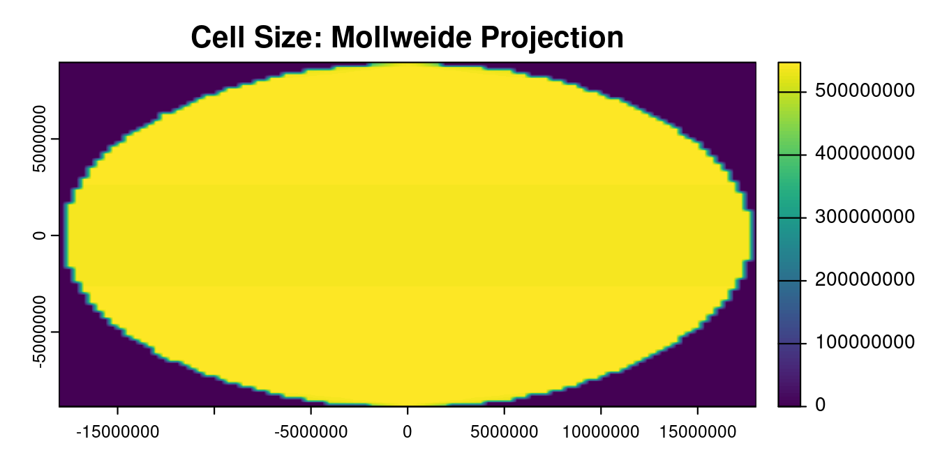
With this plot, we can see that there is a consistent cell size across globe, or that this is an equal-area coordinate reference system. Based on the cell area summary, the yellow values in the center oval of the plot (which appears to cover the extent of the data plotted in the log-transformed plot) are mostly around 547 million m².

These changes are interesting, but not unexpected for this kind of transformation. However, when we performed the same global summation calculation to determine the total sum of commercial landings in tonnes in 2017, we saw a remarkable (and concerning) difference:

# Count the total tonnes
terra::global(fish_moll, "sum", na.rm = TRUE)
# 389.3 million

                               sum
commercial_landings_2017 389271065

389 million tonnes is a much higher value than the ~87 million value calculated with the raw data!!! Reprojecting the data impacted the values to a significant degree.

When the data was projected, cell sizes changed and were also warped (increased and decreased in different areas) to be uniform across the globe. When we projected the data from EPSG:4326 to Mollweide, the count associated with one cell in the original raster was applied to multiple cells in the Mollweide CRS. This results in a large error in our data!

For example, if a raster cell near the equator had a landings value of 100 tonnes and a cell area of 1 billion m², and that raster cell in EPSG:4326 corresponded to an equivalent of 2 raster cells in Mollweide with an area of 500 million m² each, the values wouldn’t be broken into 50 tonnes in one new cell and 50 tonnes in the other. Instead, they would both appear as 100 tonnes, for a total new value of 200 tonnes.

We can tell that this type of inflation occurred based on how much higher the global summary value became. Many cells in the original raster were warped to fit into the corresponding Mollweide cells.

Solution: Convert Counts to Density

One way that we can work around this issue is to convert values from counts to density before projecting our data to a new CRS. This way, density will still be accurate, even if cell sizes change. If we need the final units to be in tonnes, we can multiply the density by the new cell size to get counts again.

In the following chunk, we will calculate the density of commercial landings (in tonnes) per cell area (in m²). We’ll then project this density raster from EPSG:4326 to Mollweide. The code for defining the cell_area and moll objects are the same as they were in earlier code chunks and are repeated here for reference.

# find size (area in square meters) of data in original crs
cell_area <- terra::cellSize(fish)

# get density (tonnes/area)
fish_density <- fish / cell_area

# define Mollweide CRS specifications
moll <- "+proj=moll +lon_0=0 +x_0=0 +y_0=0 +datum=WGS84 +units=m +no_defs"

# reproject to Mollweide
fish_density_moll <- terra::project(fish_density, crs(moll))

We can now find the area of the new cells using terra::cellSize() and multiply this by the projected density values to get counts (commercial landings in tonnes, our original units).

# get area of cells
new_cell_size <- terra::cellSize(fish_density_moll)


# multiply density by area to get count (tonnes)
new_tonnes <- fish_density_moll * new_cell_size

To check if this density-to-counts approach avoids the same errors that projecting the data without converting to density caused, we will perform a final global operation to get the total sum of all commercial landings values in the raster. This is one of those moments where we cross our fingers and hope this new approach solves the error!

# sum to check
terra::global(new_tonnes, "sum", na.rm = TRUE)
#> ~85 million!

                              sum
commercial_landings_2017 85253920	

This total value is now around 85 million! Yay! While this is not exactly the same as the value we calculated in the original data (86 million), is significantly closer to it than the value of 389 million that we got by simply projecting the commercial landings (counts) data.

This shows that converting counts to density before projecting to a new CRS is absolutely required if you do not want to introduce a massive error in your data. If we had not converted to density before projecting the data to Mollweide, and continued to reproject to another CRS, the data would continue to be warped and transformed, echoing the original mistake.

Beyond the potential for errors, density (e.g., tonnes/m²), can be visually less biased than counts (e.g., tonnes) because it automatically controls for differences in cell sizes when working with lat/lon CRS (or, any unequal area CRS).

References

Duncan, D. (2024). Ensuring Accuracy in Spatial Analysis. Ocean Health Index. https://oceanhealthindex.org/news/crs_deep_dive/

National Oceanic and Atmospheric Administration. (n.d.). Commercial fishing (Landings and revenue). NOAA Fisheries Ecosystem and Socioeconomic Indicators. https://ecowatch.noaa.gov/thematic/commercial-landings#:~:text=Commercial%20landings%20are%20the%20weight,processed%2C%20and%20sold%20for%20profit

Sea Around Us. (2024). Catches by Fishing sector in the Global Ocean [Data visualization]. Retrieved September 10, 2024, from https://www.seaaroundus.org/data/#/global?chart=catch-chart&dimension=sector&measure=tonnage&limit=10

Vox. (2016). Why all world maps are wrong [Video]. YouTube. https://www.youtube.com/watch?v=kIID5FDi2JQ

Watson, R. (2017). A database of global marine commercial, small-scale, illegal and unreported fisheries catch 1950–2014. Scientific Data, 4, 170039

Xiao, N. (2017). Map projections [Data visualization]. https://ncxiao.github.io/map-projections/index.html

News Card Image: Photo by The New York Public Library on Unsplash

Banner Image: Photo by Adolfo Félix on Unsplash